Complex-shaped Buildings - Corner Cut#
1. Project Description#
The current study numerically reproduces the experiment CornerCut_Cat2 from the Tokyo Polytechnic University (TPU) Aerodynamic Database with AeroSim’s CFD solver. The experimental results of this case, along with many other complex high-rise building geometries, are discussed in Tanaka et al.[1].
A high-rise building with \(B \times H\) dimensions:
is positioned in a wind tunnel setup with 184 pressure probes distributed over its surface:
The wind directions chosen to be simulated were:
Wind direction |
0 \(^\circ\) |
15 \(^\circ\) |
30 \(^\circ\) |
45 \(^\circ\) |
2. Simulation Setup#
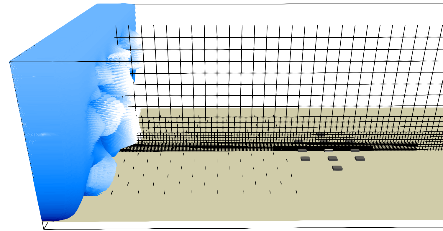
The Synthetic Eddy Method (SEM) boundary condition is applied at the inlet of the computational domain. Solid fins are distributed across the floor to ensure the desired velocity and turbulence profiles during flow development length. A Neumann boundary condition is applied at the remaining boundaries.
The building is positioned \(48B\) from inlet, and 6 grid refinement levels (\(lvl\,0\) to \(lvl\,5\)) were adopted:
A 1:2 refinement ratio is estabilished between levels, and the simulation parameters at grid \(lvl\,5\) were:
\(\boldsymbol{\Delta x/B}\) (spatial resolution) |
1.00e-02 |
\(\boldsymbol{\Delta t/CTS}\) (temporal resolution) |
6.96e-04 |
exports/\(\boldsymbol{CTS}\) (pressure acquisition frequency) |
1.00e+01 |
\(\boldsymbol{T/CTS}\) (statistical sample size) |
8.40e+02 |
\(\boldsymbol{Re_{B}=U_{H}B/\nu}\) |
4.15e+04 |
The equivalent parameters in full scale are:
\(\boldsymbol{\Delta x[m]}\) |
0.50 |
\(\boldsymbol{\Delta t[ms]}\) |
0.50 |
\(\boldsymbol{f[Hz]}\) |
14.00 |
\(\boldsymbol{T[s]}\) |
600.00 |
The computational resources required were:
Device |
NVIDIA A10G |
NVIDIA A10G |
NVIDIA A10G |
NVIDIA A10G |
Wind direction |
0 \(^\circ\) |
15 \(^\circ\) |
30 \(^\circ\) |
45 \(^\circ\) |
Node count (million) |
130.73 |
133.70 |
134.52 |
132.49 |
Allocated memory (Gb) |
18.89 |
19.33 |
19.46 |
19.18 |
Ellapsed time (h) |
44.30 |
46.94 |
48.24 |
48.45 |
3. Inflow#
An empty domain simulation is performed to measure the incident velocity and turbulence profiles. A probe line is placed at the position where the building will be located. The average velocities used for calculating the pressure coefficient and convective time scale are taken from this simulation.
Wind Profiles#
Wind Spectra#
The power spectral density of the velocity components at height \(H\) are compared with theoretical Von Kármán curves to validate the atmospheric flow.
4. Results: Local Statistics#
The pressure coefficient is calculated using the velocity at the building height \(H\) and the reference pressure measured from a position far above the building. The same statistical processing of the pressure coefficient \(C_{p}\) at each probe position is performed for both experimental and numerical data:
A sample of size (\(T / CTS\)) is evaluated over moving averages of the original signals, with window size of 3s.
The processed data is subdivided in 10 intervals, from which the minimum and maximum values will be taken for each.
Those min/max values are fitted to a Gumbel distribution.
The shape parameters from Gubel distribution are then rescaled to 3600s.
Scatter on Points Statistics#
The deviation between numerical and experimental data is quantified using the mean absolute error (MAE) and the normalized mean absolute error (NMAE):
Mean and Peak Pressures#
RMS Pressures#
Skewness and Kurtosis#
Pressure Spectrum#
Execution Notes#
Execution Date (YYYY-MM-DD) |
2025-2-26 |
Solver Version |
1.6.18 |
Changelog#
30 Oct 2024: Added scattering plots

