International RS Airport Terminal#
1. Project Description#
The current study numerically reproduces a wind tunnel assessment of International RS Airport Terminal with AeroSim’s CFD solver.
The building has \(B \times W \times H\) dimensions in full-scale:
For the current analysis, 124 pressure probes distributed across the rooftop surface were selected:
The wind directions chosen to be simulated were:
Wind direction |
0.0 \(^\circ\) |
23.0 \(^\circ\) |
45.0 \(^\circ\) |
68.0 \(^\circ\) |
90.0 \(^\circ\) |
2. Simulation Setup#
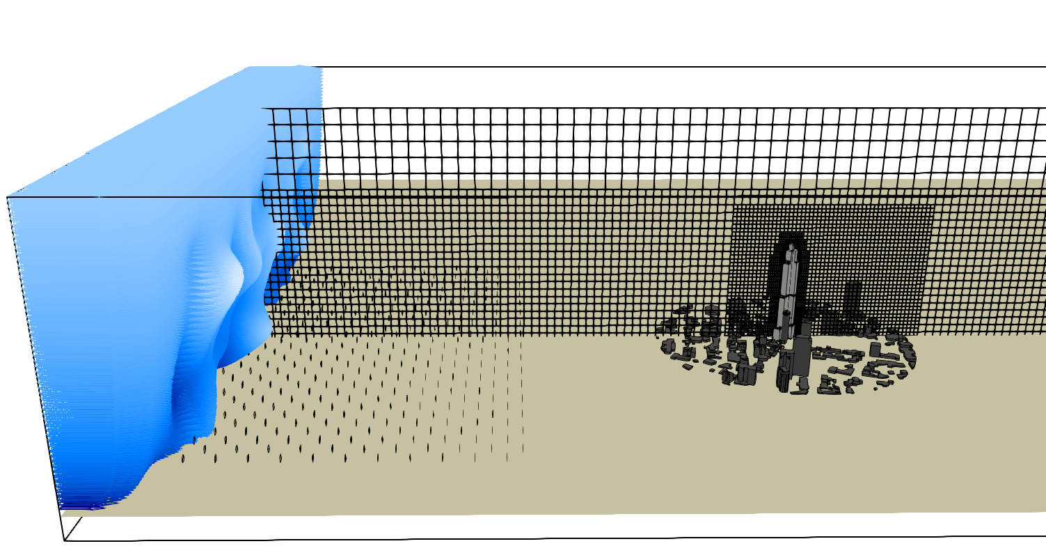
The Synthetic Eddy Method (SEM) boundary condition is applied at the inlet of the computational domain. Solid fins are distributed across the floor to ensure the desired velocity and turbulence profiles at the test section. A Neumann boundary condition is applied at the remaining boundaries.
The building is positioned \(55H\) from inlet, and 6 grid refinement levels (\(lvl\,0\) to \(lvl\,5\)) were adopted:
A 1:2 refinement ratio is estabilished between levels, and the simulation parameters at the building level were:
\(\boldsymbol{\Delta x/B}\) (spatial resolution) |
1.20e-02 |
\(\boldsymbol{\Delta t/CTS}\) (temporal resolution) |
5.78e-04 |
exports/\(\boldsymbol{CTS}\) (pressure acquisition frequency) |
1.00e+01 |
\(\boldsymbol{T/CTS}\) (statistical sample size) |
5.16e+02 |
\(\boldsymbol{Re_{H}=U_{H}H/\nu}\) |
1.49e+05 |
The equivalent parameters in full-scale are:
\(\boldsymbol{\Delta x[m]}\) |
0.50 |
\(\boldsymbol{\Delta t[ms]}\) |
0.67 |
\(\boldsymbol{f[Hz]}\) |
8.60 |
\(\boldsymbol{T[s]}\) |
600.00 |
The computational resources required were:
Device |
NVIDIA A10G |
NVIDIA A10G |
NVIDIA A10G |
NVIDIA A10G |
NVIDIA A10G |
Wind direction |
0.0 \(^\circ\) |
23.0 \(^\circ\) |
45.0 \(^\circ\) |
68.0 \(^\circ\) |
90.0 \(^\circ\) |
Node count (million) |
135.34 |
136.07 |
136.29 |
135.96 |
135.34 |
Allocated memory (Gb) |
17.93 |
18.03 |
18.06 |
18.01 |
17.93 |
Ellapsed time (h) |
20.64 |
20.81 |
20.99 |
20.61 |
20.65 |
3. Inflow#
An empty domain simulation is performed to measure the incident velocity and turbulence profiles. A probe line is placed at the position where the building will be located. The average velocities used for calculating the pressure coefficient and convective time scale are taken from this simulation.
Wind Profiles#
Length Scale#
The length scale is calculated using the autocorrelation of the longitudinal velocity. Its value is used to reescale the simulated time scale to match the experiment.
Wind Spectra#
The power spectral density of the velocity components at height \(H\) are compared with theoretical Von Kármán curves to validate the atmospheric flow.
4. Results: Local Statistics#
The pressure coefficient is calculated using the mean velocity at the building height \(H\) and the reference pressure measured from a position far above the building. For the peak pressure coefficients, the following procedure was applied for both datasets (numerical experimental):
The sample is subdivided in sub-samples of duration \(T\), and a 3s moving-average is applied to all sub-samples.
The smoothed sub-samples are divided in 10 intervals, from which the minimum and maximum values are taken.
The max/min values are fitted into a Gumbel distribution, and the mode \(U\) is rescaled to a duration of 1h.
A non-excedence probability of 78% is considered for the extreme values.
Scatter on Local Statistics#
The dispersion between numerical and experimental data is quantified using the mean absolute error (MAE) and the normalized mean absolute error (NMAE):
Mean and Peak Pressures#
The extreme values range for the experimental data is delimited by the sub-samples of duration \(T\).
RMS Pressures#
Skewness and Kurtosis#
Pressure Spectrum#
Execution Notes#
Execution Date (YYYY-MM-DD) |
2025-3-5 |
Solver Version |
1.6.18 |
Changelog#
30 Oct 2024: Added scattering plots

